But the cells contained in rows or columns might eventually be useful later, or they might contain information that is part of a formula and needs to be updated. In these scenarios, it is essential that the hidden cells be unhidden so that they can be modified. Fortunately you can follow a few simple steps to unhide all of the rows and columns in an Excel 2013 spreadsheet that have previously been hidden.
View All of the Hidden Cells in Microsoft Excel 2013
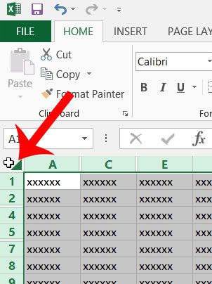
The steps in this tutorial will show you how to show all of the rows and columns in your Excel spreadsheet that are currently hidden. Individual cells cannot be hidden, so you will need to unhide the row or column that contained the hidden information that you need to view. You can read this article to learn how to selectively unhide just a single row or column instead. Otherwise, continue below. Step 1: Open your spreadsheet in Excel 2013. Step 2: Click the cell at the top-left corner of the spreadsheet.
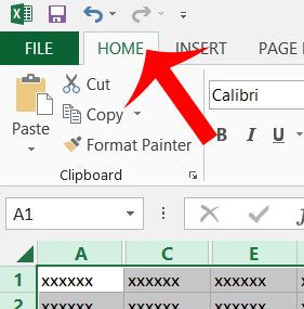
Step 3: Click the Home tab at the top of the window.
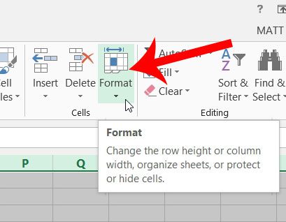
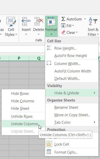
Step 4: Click the Format drop-down menu in the Cells section of the navigational ribbon.
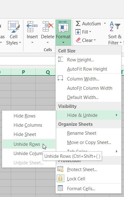
Step 5: Click the Hide & Unhide option, then click Unhide Rows.
Step 6: Repeat steps 4 and 5, but click the Unhide Columns option instead.
Are there rows or columns in your spreadsheet that you would like to hide? Read here and learn how. After receiving his Bachelor’s and Master’s degrees in Computer Science he spent several years working in IT management for small businesses. However, he now works full time writing content online and creating websites. His main writing topics include iPhones, Microsoft Office, Google Apps, Android, and Photoshop, but he has also written about many other tech topics as well. Read his full bio here.
You may opt out at any time. Read our Privacy Policy
