One way that you can make sure you see things, such as numbers that are less than zero, is by making them look different. A common way to achieve this is by making the values a different color. Our tutorial below will show you how to apply conditional formatting to cells in Google Sheets so that their values will be red if they are less than zero.
How to Make Google Sheets Values Red When Less Than Zero
Our guide continues below with additional information on how to make cells red if a number is less than zero in Google Sheets, including pictures of these steps. Microsoft Excel shares many of the features of Google Sheets, including formulas. Check out this Excel subtraction formula article to find out more about subtracting cell values. In Microsoft Excel, there is a number formatting option where you can have Excel automatically change the color of a number to red if the value of that number is less than zero. This is very helpful for many situations where you might use Excel, so if you are formatting a spreadsheet in Google Sheets, you may be looking for a way to achieve this. One way to accomplish it is with Google Sheets’ conditional formatting. Our guide below is going to show you how to select a range of cells, then apply conditional formatting to that range so that Google Sheets will automatically change the fill color of a cell to red if the value in that cell is less than zero. You can make similar adjustments in Excel, too. Our tutorial on how to make n/a zero in Excel can show you how to reduce errors with the VLOOKUP formula.
How to Use Google Sheets Conditional Formatting to Change Cell Color (Guide with Pictures)
The steps in this article were performed in the desktop version of the Google Chrome Web browser, but will also work in other desktop browsers like Firefox or Edge.
Step 1: Sign into your Google Drive at https://drive.google.com and open the file to which you want to apply the formatting.
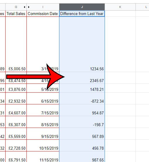
Step 2: Select the range of cells containing the values to modify.
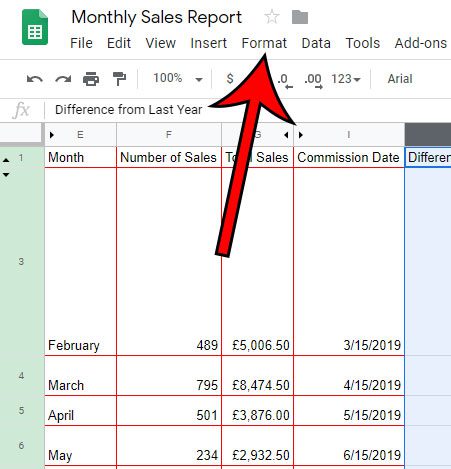
Step 3: Click the Format tab at the top of the window.
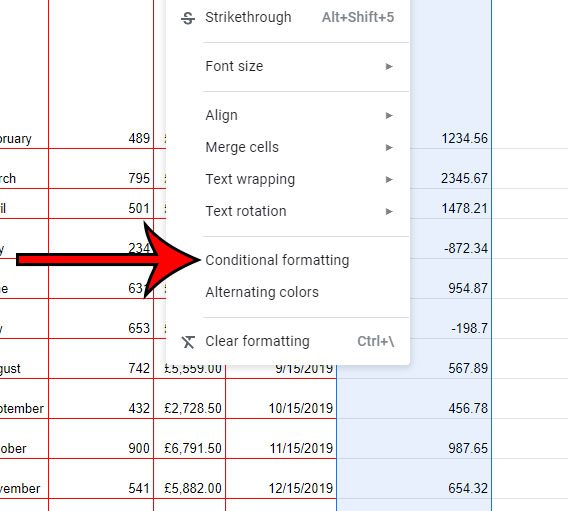
Step 4: Choose the Conditional formatting option at the bottom of the menu.
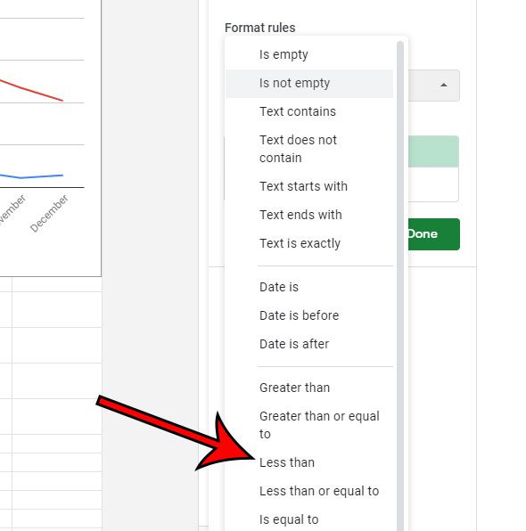
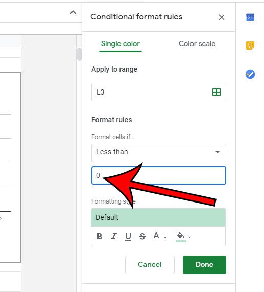
Step 5: Click the Format cells if dropdown menu, then choose the Less than option.
Step 6: Type “0” into the Value or formula field.
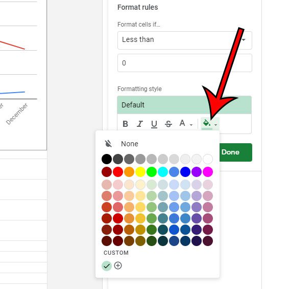
Step 7: Click the Fill color button, then choose red, or the desired color.
Note that there is a Text color button to the left of this if you would rather just make the text color red.
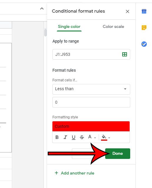
Step 8: Click the Done button.
Now that you know how to display values in red if they are less than zero in Google Sheets, you can use this technique for other types of conditional formatting as well. Are you working on a file with a number of other people, and you’re tired of constantly checking to see if someone has made a change or a comment? Find out how to enable change notifications in Google Sheets so that you can receive an email when changes occur instead. After receiving his Bachelor’s and Master’s degrees in Computer Science he spent several years working in IT management for small businesses. However, he now works full time writing content online and creating websites. His main writing topics include iPhones, Microsoft Office, Google Apps, Android, and Photoshop, but he has also written about many other tech topics as well. Read his full bio here.
