One such setting involves configuring a row so that it is always visible. This makes it much easier to identify cell data. Our tutorial below will show you how to do this by learning how to lock a row in Google Sheets.
How to Freeze a Row in Google Sheets
Our article continues below with additional information on how to lock a row in Google Sheets, including pictures of these steps. Have you ever been working a spreadsheet that someone else created, only to notice that the top row on the sheet wasn’t moving as you scrolled down? The ability to lock the row in place like this is very helpful, especially when you have large spreadsheets with similar types of data. Google Sheets shares many of the same features found in Microsoft Excel that improve the usability of the application for both the creator and the people viewing the file. Since a premium is often placed on creating the data and getting it right, functionality and printing often take a back seat. One way that you can help ensure that data entry is accurate, and that readers don’t become confused, is to lock your header row, or title row, to the top of the sheet. Our guide below will show you how to lock a Google Sheets row so that it remains visible on the computer screen, and also prints on each page of the spreadsheet if you need a copy of your data on paper, too.
How to Lock a Header or Title Row in a Google Spreadsheet (Guide with Pictures)
The steps in this article were performed in the desktop version of the Google Chrome Web browser, but will also work in other desktop browsers like Mozilla Firefox or Apple Safari. You can access your Google Sheets files here. Now that you know how to lock a row in Google Sheets you will be able to do this for any future spreadsheet that you edit which would benefit by keeping your header row visible at the top of the worksheet. This method is probably the easiest way to lock a Google Sheets row, but it may not be the fastest. If you find that you are locking rows a lot, then you may wish to learn the alternate method below.
Method 2 – How to Lock Rows in Google Sheets
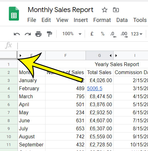
There is an alternate method for locking rows in Google Sheets that many people find to be more convenient. In the cell above the row 1 heading and to the left of the column A heading there is a horizontal gray bar. If you click and drag that bar down you will be able to lock all of the rows above that bar. The steps in the tutorial above are going to cause the frozen row, or rows, to remain visible at the top of the window as you scroll down. You can use this functionality to easily identify the column in which you are adding or editing data, which can be useful in helping to avoid mistakes.
More Information on How to Lock a Row in Google Sheets
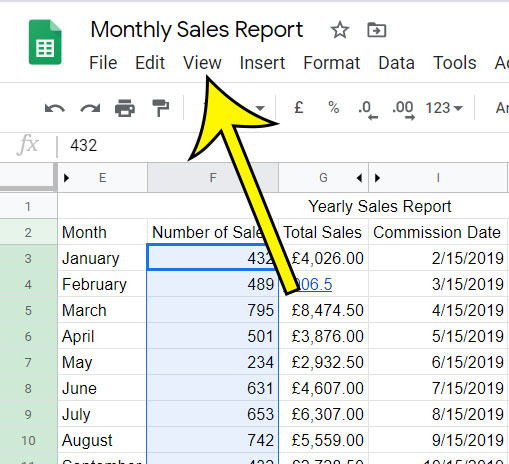
Large spreadsheets can be difficult to manage as you begin to add more and more rows of data. Constantly having to scroll back up to the top of the spreadsheet to see what data belongs in which columns can be tedious and error-prone. Fortunately you can lock a row in Google Sheets so that it stays visible at the top of the page, even when it should be hidden from view as you scroll down. The steps in the guide above discuss low to lock, or how to freeze, rows in Google Sheets using an option found on the “View” menu. While choosing to freeze a single row or column, or multiple rows or columns is important for your work in the app, you might also want to freeze the top row or left column in Google Sheets when you print. To accomplish this go to File > Print then select the Headers & footers tab at the right side of the window. You can then scroll down and check either the Repeat frozen rows or Repeat frozen columns option to repeat those frozen groups of cells on each page of the printed spreadsheet.
Difference Between Locking Rows and Columns in Google Sheets
There are many different ways to format a spreadsheet in Google Sheets, so locking a row may not be helpful to you. But if you place descriptions in the first column instead of the first row, then you can use a similar method to lock that column to the left side of the window, Rather than choosing the row freezing options at the top of the “Freeze” menu you can select the column freezing options at the bottom of the menu.
Conclusion
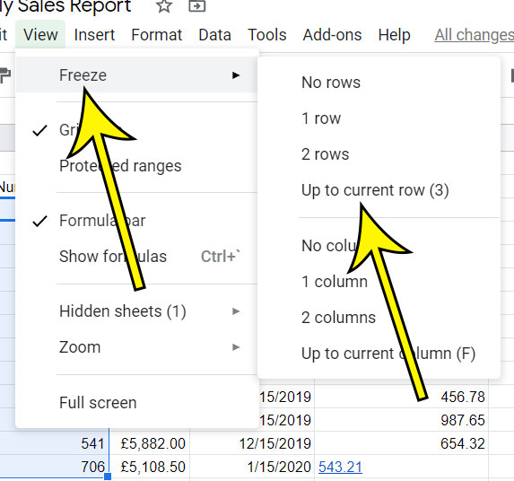
Now that you know how to freeze or lock rows in Google Sheets you can take advantage of it to improve your own experience in the application, as well as the experience of others that will be looking at your data. Simply click View at the top of the window, then Freeze, then choose the No rows option. Additionally, by combining this feature with some of the other options found on the print menu you can create a physical copy of your spreadsheet that will be easier to understand and identify.
Additional Reading
How to change the orientation of a printed spreadsheet in Google SheetsHow to sort a column from high to low in Google SheetsHow to print with gridlines in Google SheetsHow to copy multiple rows in Google SheetsHow to change cell border color in Google Sheets
He specializes in writing content about iPhones, Android devices, Microsoft Office, and many other popular applications and devices. Read his full bio here.