Hiding columns or rows in Excel is the perfect solution to this situation, as your data is still technically part of the spreadsheet, and any formulas that reference cells contained within those hidden rows or columns will still display properly. But a hidden row will not be visible when the spreadsheet is printed or viewed on a computer screen, allowing you to focus the attention of your readers on the data that you have chosen to leave visible.
Hiding a Row in Microsoft Excel 2013
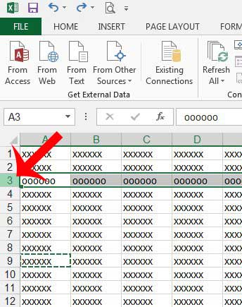
The steps below were written for Microsoft Excel 2013, and the images are of Microsoft Excel 2013. However, these steps will work for earlier versions of Excel as well. Step 1: Open the spreadsheet in Excel 2013 that contains the row that you want to hide. Step 2: Click the row number at the left of the spreadsheet to select the row that you want to hide. I am hiding row 3 in the example image below.
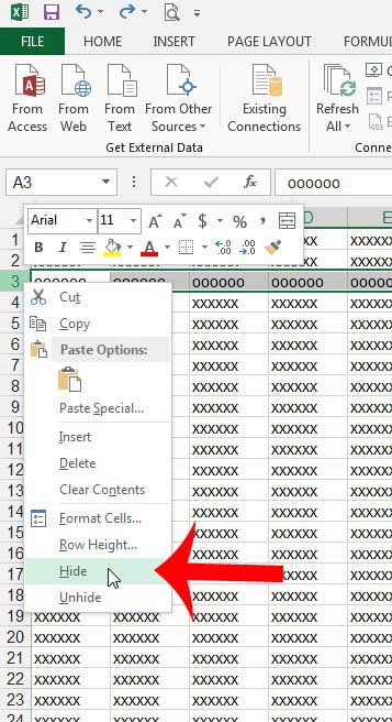
Step 3: Right-click the row number, then click the Hide option.
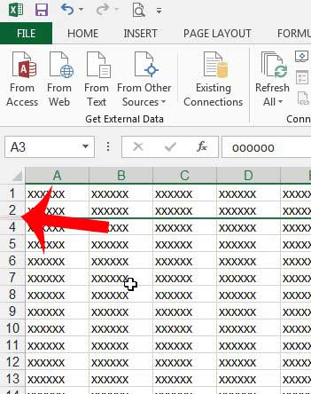
The numbering of your rows should now skip the row that you just hid.
You can learn how to unhide a hidden row or column by following the steps in this article. Are you printing a large spreadsheet that is difficult to follow on each page due to a lack of column headings? Learn how to print the top row of your spreadsheet on every page in Excel 2013 to make the data on each page simpler to read. After receiving his Bachelor’s and Master’s degrees in Computer Science he spent several years working in IT management for small businesses. However, he now works full time writing content online and creating websites. His main writing topics include iPhones, Microsoft Office, Google Apps, Android, and Photoshop, but he has also written about many other tech topics as well. Read his full bio here.
You may opt out at any time. Read our Privacy Policy