Have you ever worked on a large spreadsheet where you needed to keep scrolling back up to the top of the sheet to make sure that you were looking at the right column? This can be frustrating and time-confusing, while also potentially leading to mistakes. Luckily you can fix this problem by learning how to freeze a row in Microsoft Excel. This will keep a row (such as the row with your headings) visible at the top of the screen at all times. Our guide below will show you how to enable this option in your spreadsheet. This article is split into several sections. You can click any of the links below to go directly to the section that interests you, or you can keep scrolling to read the entire article.
How to Make the Top Row Stay in Excel
Our article continues below with additional information on freezing rows in Microsoft Excel, including pictures of these steps.
How Do You Freeze a Row in Excel? (Guide with Pictures)
The steps in this article were performed in Microsoft Excel for Office 365, but will also work in most other versions of Excel. Note that this setting must be applied individually to each spreadsheet that you edit. By freezing a row using the steps in this section you will be able to freeze either the top row of your spreadsheet, or several of the top rows of the spreadsheet.
Step 1: Open your spreadsheet in Excel.
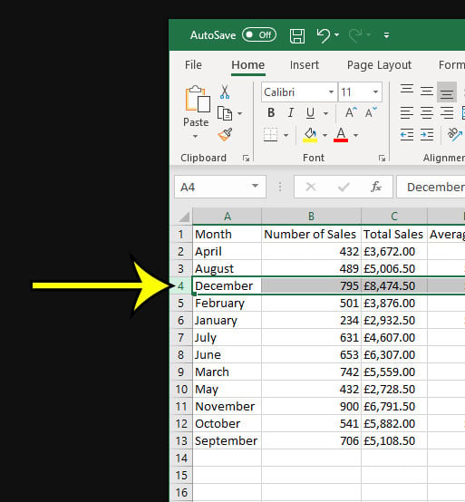
Step 2: Click the row number at the left of the spreadsheet that is under the row(s) that you wish to freeze.
I am going to be freezing the top three rows of my sheet in the picture below.
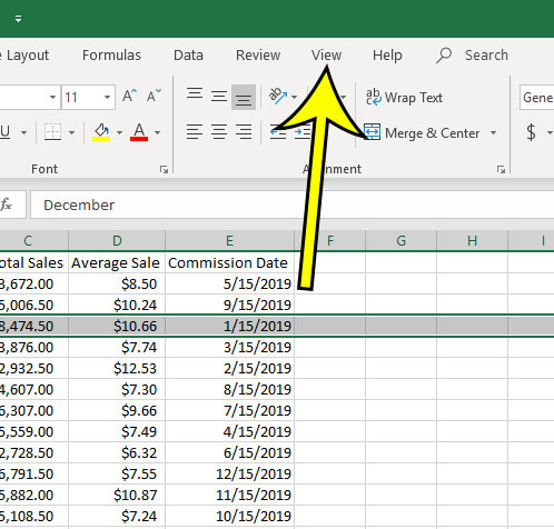
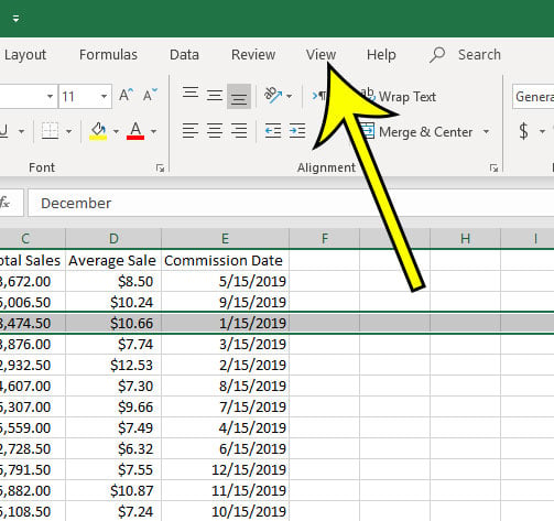
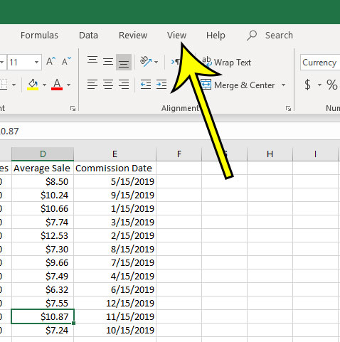
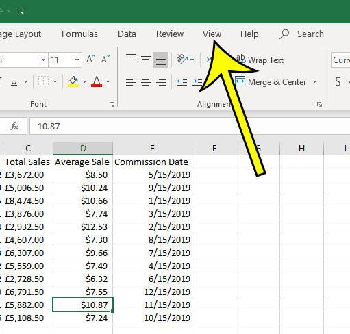
Step 3: Select the View tab at the top of the window.
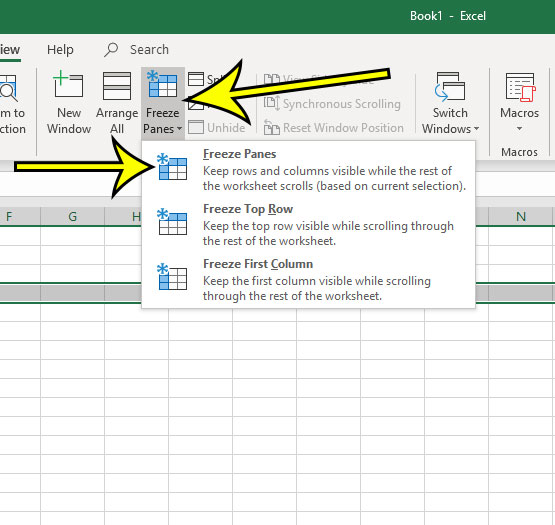
Step 4: Choose the Freeze Panes button, then click the Freeze Panes button.
Can You Freeze Any Row in Excel? (Guide with Pictures)
Using the Freeze Panes option in the section above will allow you to freeze either the top row of the spreadsheet by itself, or several of the top rows on the spreadsheet. But what if you want to freeze just one of the rows in the middle of your spreadsheet? While this isn’t possible using the Freeze Panes tool, you can get close to what you want using the Split feature. Make sure that you don’t have an entire row or column selected before completing the steps in this section, as that will affect what the Split function does to your sheet.
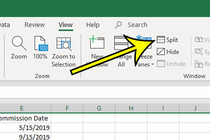
Step 1: Select the View tab at the top of the window.
Step 2: Click the Split button.
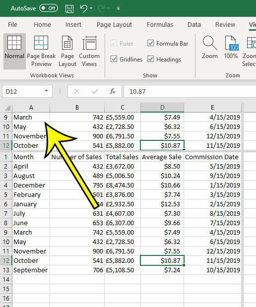
This is going to segment the spreadsheet into four sections.
Step 3: Click inside the top-left window, then use the arrow keys or scroll so that the row that you wish to “freeze” is the top row in this section.
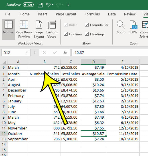
I am going to freeze row 9 of my sheet in the image below.
Step 4: Drag the horizontal split bar so that only the top row of the top-left section is visible.
You can now click inside the bottom-left window and navigate through the sheet while keeping that middle row “frozen” in the top window.
How Do You Make the Top Row in Excel Stay? (Guide with Pictures)
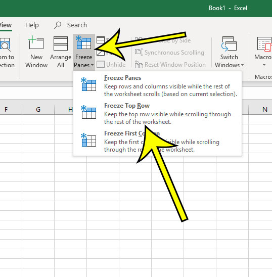
While you can freeze the top row of your spreadsheet using the Freeze Panes method described in the first section of this article, there is another way to accomplish the desired result that lets you skip the step of selecting a row number.
Step 1: Click the View tab at the top of the window.
Step 2: Click the Freeze Panes button, then choose the Freeze Top Row button.
How Do I Unfreeze a Row in Excel? (Guide with Pictures)
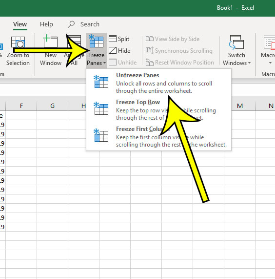
Now that you’ve discovered how to freeze a row in Excel, you may be wondering how to undo it should you be working on a spreadsheet that has a frozen row you don’t want.
Step 1: Click the View tab.
Step 2: Select the Freeze Panes button, then click the Unfreeze Panes option.
If you are also a Google Docs user, then find out how to freeze the top row in Google Sheets and get the same functionality in Google’s Web-based spreadsheet application.
Additional Reading
He specializes in writing content about iPhones, Android devices, Microsoft Office, and many other popular applications and devices. Read his full bio here.
